A practical introduction to approximate Bayesian computation
Introduction
In this tutorial, we’ll learn the basics of approximate Bayesian computation (ABC). ABC is a very flexible inference method that is quite intuitive, and that you can apply to almost any model type. As such, it is quite handy to have it in one’s toolbox! To build up an intuition of the method, we’ll perform ABC on a very simple ecosystem model, using Julia, and will visualize graphically the inference results.
Package loading
We first need to load a few packages.
cd(@__DIR__)
using Pkg; Pkg.activate(".")
using Random
using LinearAlgebra
import Optimisers:destructure # required to simplify parameter indexing
using UnPack # for parameter indexing
using ApproxBayes # ABC toolbox
using Distributions # useful to define the priors
using OrdinaryDiffEq # ODE solver library
using ParametricModels # convenience package for ODE models. /!\ package not registered
It is always important to make your work reproducible, so we’ll set manually a seed to the random number generator.
# Set a seed for reproducibility.
Random.seed!(11);
Model definition and data generation
What we’ll do is to implement an Ordinary Differential Equation model, which will be used to generate synthetic data and further perform the inference. The idea here is to consider this synthetic data as our empirical data, and pretend that we do not know which parameters generated this data. Our goal is then to recover the generating parameters.
We’ll consider a predator-prey ecological model, the Lotka-Volterra equations. This model has a total of four different parameters $\alpha, \beta, \gamma, \delta$, that describe the interactions between the two species. For the sake of simplicity, we’ll assume that we know perfectly the parameters $\gamma, \delta$, and seek to infer $\alpha$ and $\beta$. Assuming to know $\gamma, \delta$ is of course a very unrealistic assumption… but a handy assumption to develop an intuition about parameter inference.
We use ParametricModels.jl to define our model. ParametricModels.jl is a simple wrapper around OrdinaryDiffEq.jl, that allows to play around with the model without bothering further about the details of the numerical solve. This makes it easier to simulate repeatedly an ODE model. For readability and maintenance, we’ll encapsulate the parameters in a NamedTuple.
# Declaration of the model
ParametricModels.@model LotkaVolterra
# Definition of the model
function (lv::LotkaVolterra)(du, u, p, t)
    # Model parameters
    @unpack α, β, = p
    # Current state
    x, y = u
    # fixed parameters
    γ = 3.0
    δ = 1.0

    # Evaluate differential equations
    du[1] = (α[] - β[] * y) * x # prey
    du[2] = (δ * x - γ) * y # predator

    return nothing
end
# Define initial-value problem.
u0 = [1.0, 1.0]
p = (α=[1.5], β=[1.0])
tspan = (0.0, 10.0)

model = LotkaVolterra(ModelParams(;u0, p, tspan, alg=Tsit5(), saveat=0.1))
sol = simulate(model);
And here we go, we have our model defined!
As an exercise, you could try to write the same model with OrdinaryDiffEq.jl.
Let’s now plot the model output. We first need to import some plotting utilities. For plotting, I tend to use PyPlot.jl, which is a wrapper around the Python library matplotlib. I find it much more convenient than the Julia package Plots.jl, in the sense that it contains more utility functions. It is always a good idea to load in parallel PyCall.jl, which allows to import other utility funtions from Python.
using PyPlot # to plot 3d landscape
using PyCall
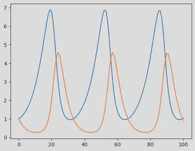
Here is a plot of the model output without noise:
fig = PyPlot.figure()
PyPlot.plot(sol')
display(fig)
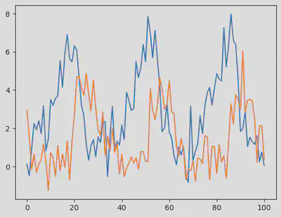
We now use sol to generate synthetic data containing some noise (in mathematical terms, we call this a Gaussian white noise, which follows $\mathcal{N}(0,\sigma)$ where $\sigma = 0.8$.
σ = 0.8
odedata = Array(sol) + σ * randn(size(Array(sol)))
fig = figure()
PyPlot.plot(odedata')
display(fig)
The model and the synthetic data are ready, let’s get started with ABC!
Approximate Bayesian computation
For ABC, one needs to define a function $\rho$ that measures the distance between the model output $\hat \mu$ (in the picture below, $\mu_i$) and the empirical data $\mu$.

In our case, the empirical data available (odedata) allows us to explicitly define the likelihood of the model given the data. As a distance function, we therefore can first use the negative log of the likelihood. For additive Gaussian noise, the likelihood of the model is given by
$$\begin{split} p(y_{1:K} | \theta, \mathcal{M}) &= \prod_{i=1}^K p(y_{i} | \theta, \mathcal{M})\\ &= \prod_{k=1}^K \frac{1}{\sqrt{(2\pi)^d|\Sigma_y|}} \exp \left(-\frac{1}{2} \epsilon_k^{T} \Sigma_y^{-1} \epsilon_k \right) \end{split}$$
where $\epsilon_k \equiv \epsilon(t_k) = y(t_k) - h\left(\mathcal{M}(t_k, \theta)\right)$ and $\Sigma_y = \sigma^2 I$ in our case.
So let’s translate all this in Julia code.
ApproxBayes.jl requires as input a function simfunc(params, constants, data), which plays the role of the $\rho$ function. It should return the distance value, as well as a second value that may be used for logging. To make things simple, we’ll return nothing for this second value.
Because ApproxBayes.jl requires that params is an array (params <: AbstractArray), we further use a special trick relying on the function Optimiser.destructure. This utility function allows to generate a function re that can recover a NamedTuple from a vector. Very useful in combination with the utility macro @unpack!
_, re = destructure(p)
function log_likelihood(p; odedata=odedata)
    p_tuple = re(p)
    pred = simulate(model, p=p_tuple)
    return sum([loglikelihood(MvNormal(zeros(2), LinearAlgebra.I * σ^2), odedata[:,i] - pred[:,i]) for i in 1:size(odedata,2)])
end
function simfunc(params, constants, data)
    ρ = - log_likelihood(params, odedata=data)
    return ρ, nothing
end

# testing function
simfunc([1.0, 1.2], nothing, odedata)
(1403.0830673958446, nothing)
Now that the distance function is implemented, we define the priors on the parameters $\alpha, \beta$
priors = [truncated(Normal(1.1, 1.), 0.5, 2.5), # for α and β
            truncated(Normal(1.1, 1.), 0., 2.)]
num_samples = 500
max_iterations = 1e5
ϵ = 2.0
abcsetup = ABCRejection(simfunc,
                        length(priors),
                        ϵ,
                        ApproxBayes.Prior(priors);
                        nparticles=num_samples,
                        maxiterations=max_iterations)

abcresult = runabc(abcsetup, odedata, progress=true, parallel=true)
Preparing to run in parallel on 5 processors
Number of simulations: 1.00e+05
Acceptance ratio: 5.00e-03

Median (95% intervals):
Parameter 1: 1.51 (1.48,1.53)
Parameter 2: 1.00 (0.86,1.16)
And here we go: abcresult informs us that the ABC inference could indeed recover the parameters that generated the data!
Visualizing the inference process
To better understand what has happened, let’s plot the parameters that have been accepted by the sampler, together with the real likelihood landscape. As a first step, let’s visualise the real likelihoood landscape.
αs = range(1.45, 1.55, length=100)
βs = range(0.8, 1.3, length=100)
likelihoods = Float64[]
for α in αs
    for β in βs
        p = [α, β]
        push!(likelihoods, log_likelihood(p))
    end
end

likelihoods = exp.(likelihoods); # exponentiating, to make it visually nicer
We now define an Axes3D, as you would do it in Python:
# Plotting 3d landscape
fig = plt.figure()
ax = Axes3D(fig, computed_zorder=false);
We’ll import numpy into Julia, to easily construct the meshgrid required by the matplotlib function plot_surface.
np = pyimport("numpy") # used for plotting
X, Y = np.meshgrid(αs, βs)


# fig.savefig("perturbed_p.png", dpi = 300, bbox_inches="tight")
ax.plot_surface(X .|> Float64,
    Y .|> Float64,
    reshape(likelihoods, (length(αs), length(βs))) .|> Float64,
    edgecolor="0.7",
    linewidth=0.2,
    cmap="Blues", zorder=-1)
ax.set_xlabel(L"p_1")
ax.set_ylabel(L"p_2")
ax.set_zlabel("Likelihood", x=2)
ax.set_xticks([])
ax.set_yticks([])
ax.set_zticks([])

# make the panes transparent
ax.xaxis.set_pane_color((1.0, 1.0, 1.0, 0.0))
ax.yaxis.set_pane_color((1.0, 1.0, 1.0, 0.0))
ax.zaxis.set_pane_color((1.0, 1.0, 1.0, 0.0))
# make the grid lines transparent
ax.xaxis._axinfo["grid"]["color"] = (1.0, 1.0, 1.0, 0.0)
ax.yaxis._axinfo["grid"]["color"] = (1, 1, 1, 0)
ax.zaxis._axinfo["grid"]["color"] = (1, 1, 1, 0)

fig.tight_layout()
fig.set_facecolor("None")
ax.set_facecolor("None")

for p in eachrow(abcresult.parameters)
    ax.scatter(p[1], p[2], exp.(log_likelihood(p)), c="tab:red", zorder=100, s = 0.5)
end
p = abcresult.parameters[1,:]
ax.scatter(p[1], p[2], exp(log_likelihood(p)), c="tab:red", zorder=100, s = 2., label="Accepted simulation")
ax.legend()
display(fig)
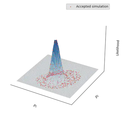
Cool, right?
Summary statistics
It may be useful, or necessary, to use summary statistics of the data instead of the full likelihood, to be provided to the distance function. Summary statistics are values calculated from the data to represent the maximum amount of information in the simplest possible form. Using summary statistics allows to reduce the dimensionality of the data, which increases the probability of accepting the model output. In our case, the dimensionality correponds to the number of time steps multiplied by the number of state variables). Using summary statistics may prove useful to improve the convergence of the inference process, were the inference not converge using the likelihood function. But because it reduces the amount of information provided to the inference method, it may also hamper a precise characterisation of the model parameter values.
Mean and variance
As summary statistics, we can here compute the mean and covariance matrix of the state variables, and use those to define the distance between the model output and the data.
compute_summary_stats(data) = [mean(data,dims=2); cov(data, dims=2)[:]]
ss_data = compute_summary_stats(odedata)
6×1 Matrix{Float64}:
 2.966416873264894
 1.5414956648089986
 4.784360022666909
 0.07385819785251807
 0.07385819785251807
 2.680060599643699
Let’s now proceed similarly to above
function simfunc(params, constants, ss_data)
    p_tuple = re(params)
    pred = simulate(model, p=p_tuple)
    ss_pred = compute_summary_stats(pred)
    ρ = sum((ss_pred .- ss_data).^2) # taking euclidean distance between
    return ρ, nothing
end

simfunc([1.0, 1.2], nothing, ss_data)

priors = [truncated(Normal(1.1, 1.), 0.5, 2.5), # for α and β
            truncated(Normal(1.1, 1.), 0., 2.)]
num_samples = 500
max_iterations = 1e5
ϵ = 0.15
abcsetup = ABCRejection(simfunc,
                        length(priors),
                        ϵ,
                        ApproxBayes.Prior(priors);
                        nparticles=num_samples,
                        maxiterations=max_iterations)

abcresult = runabc(abcsetup, ss_data, progress=true, parallel=true)
Preparing to run in parallel on 5 processors
Number of simulations: 1.00e+05
Acceptance ratio: 5.00e-03

Median (95% intervals):
Parameter 1: 2.10 (1.98,2.30)
Parameter 2: 1.11 (1.01,1.23)
As you can see, the results of the inference or much less accurate.
Which other summary statistics of the time series could you think of? You can find below tests with other summary statistics.
And that’s it for today! Hopefully this tutorial has given you some basics and intuition on ABC, and how to use in Julia.
Further references
Appendix
You can find the corresponding tutorial as a .jmd file at https://github.com/vboussange/MyTutorials. To use ParametricModels.jl, follow the procedure indicated on the github repo.
Please contact me, if you have found a mistake, or if you have any comment or suggestion on how to improve this tutorial.
Summary statistics with Fourier transforms
using FFTW
# Fourier Transform of the data
F = fft(odedata .- mean(odedata,dims=2)) |> fftshift
# freqs = fftfreq(size(odedata, 2), 1.0/Ts) |> fftshift
fig = figure()
plot(1:size(odedata,2), abs.(F)')
display(fig)
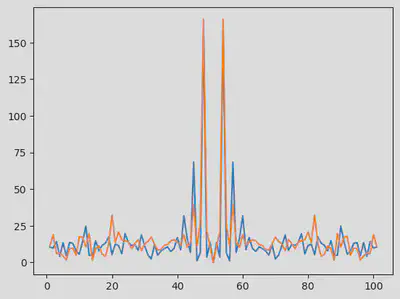
Let’s select the frequency which frequency is predominent, and consider it for our summary statistics
freq_x = sortperm(abs.(F[1,:]))[end-1:end] # selecting the two most important frequencies
freq_y = sortperm(abs.(F[1,:]))[end-1:end] # selecting the two most important frequencies
@assert freq_x == freq_y # both prey and predator data peak at the same frequencies

function compute_summary_stats(data)
    F = fft(Array(data)) |> fftshift
    return abs.(F[:,freq_x])
end
ss_data = compute_summary_stats(Array(odedata))
simfunc([1.0, 1.2], nothing, ss_data)
(29583.477061802652, nothing)
Let’s now proceed similarly to above
priors = [truncated(Normal(1.1, 1.), 0.5, 2.5), # for α and β
            truncated(Normal(1.1, 1.), 0., 2.)]
num_samples = 500
max_iterations = 1e5
ϵ = 0.15
abcsetup = ABCRejection(simfunc,
                        length(priors),
                        ϵ,
                        ApproxBayes.Prior(priors);
                        nparticles=num_samples,
                        maxiterations=max_iterations)

abcresult = runabc(abcsetup, ss_data, progress=true, parallel=true)
Preparing to run in parallel on 5 processors
Number of simulations: 1.00e+05
Acceptance ratio: 5.00e-03

Median (95% intervals):
Parameter 1: 1.44 (1.05,2.38)
Parameter 2: 0.92 (0.26,0.99)
Although we have quite a large uncertainty on the parameters, the Fourier transform-based summary statistics seem to contain more relevant information, and this is reflected on the more accurate value of the inferred parameters.
Summary statistics with auto-correlation
Here we use the autocorrelation function to build our summary statistics. The default lag value of the autocor in Julia reduces the dimension of the data to a matrix of size 21x2.
using StatsBase
autocor_ss = autocor(odedata')
fig = figure()
plot(1:size(autocor_ss,1), autocor_ss)
display(fig)
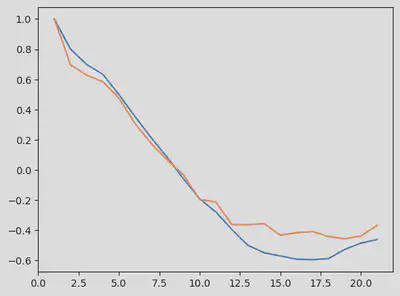
If we were to compute the lag from $t = 0$ to $t = t_{\text{max}}$, we would obtain a sinusoidal curve, similar to the time series raw data.
compute_summary_stats(data) = autocor(Array(data)')
ss_data = compute_summary_stats(odedata)
simfunc([1.0, 1.2], nothing, ss_data)
(1.4530748281677037, nothing)
Let’s now proceed similarly to above
priors = [truncated(Normal(1.1, 1.), 0.5, 2.5), # for α and β
            truncated(Normal(1.1, 1.), 0., 2.)]
num_samples = 500
max_iterations = 1e5
ϵ = 0.15
abcsetup = ABCRejection(simfunc,
                        length(priors),
                        ϵ,
                        ApproxBayes.Prior(priors);
                        nparticles=num_samples,
                        maxiterations=max_iterations)

abcresult = runabc(abcsetup, ss_data, progress=true, parallel=true)
Preparing to run in parallel on 5 processors
Number of simulations: 1.00e+05
Acceptance ratio: 5.00e-03

Median (95% intervals):
Parameter 1: 1.53 (1.45,1.61)
Parameter 2: 0.35 (0.29,0.41)