Parameter Inference in dynamical systems
One of the challenges modellers face in biological sciences is to calibrate models in order to match as closely as possible observations and gain predictive power. Scientific machine learning addresses this problem by applying optimisation techniques originally developed within the field of machine learning to mechanistic models, allowing to infer parameters directly from observation data.
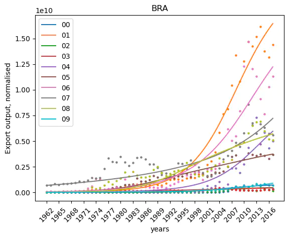 Calibrating a system of differential equations on data for the project Econobiology.
One of the challenges modellers face in biological sciences is to calibrate models in order to match as closely as possible observations and gain predictive power. This can be done via direct measurements through experimental design, but this process is often costly, time consuming and even sometimes not possible. Scientific machine learning addresses this problem by applying optimisation techniques originally developed within the field of machine learning to mechanistic models, allowing to infer parameters directly from observation data. In this blog post, I shall explain the basics of this approach, and how the Julia ecosystem has efficiently embedded such techniques into ready to use packages. This promises exciting perspectives for modellers in all areas of environmental sciences.
🚧 This is Work in progress 🚧
Dynamical systems are models that allow to reproduce, understand and forecast systems. They connect the time variation of the state of the system to the fundamental processes we believe driving it, that is
$$ \begin{equation*} \text{ time variation of } 🌍_t = \sum \text{processes acting on } 🌍_t \end{equation*} $$
where $🌍_t$ denotes the state of the system at time $t$. This translates mathematically into
$$ \begin{equation} \partial_t(🌍_t) = f_\theta( 🌍_t ) \end{equation}\tag{1} $$
where the function $f_\theta$ captures the ensembles of the processes considered, and depend on the parameters $\theta$.
Eq. (1) is a Differential Equation, that can be integrated with respect to time to obtain the state of the system at time $t$ given an initial state $🌍_{t_0}$.
$$ \begin{equation} 🌍_t = 🌍_{t_0} + \int_0^t f_\theta( 🌍_s ) ds \end{equation}\tag{2} $$
Dynamical systems have been used for hundreds of years and have successfully captured e.g. the motion of planets (second law of Kepler), the voltage in an electrical circuit, population dynamics (Lotka Volterra equations) and morphogenesis (Turing patterns)…
Such models can be used to forecast the state of the system in the future, or can be used in the sense of virtual laboratories. In both cases, one of the requirement is that they reproduce patterns - at least at a qualitative level. To do so, the modeler needs to find the true parameter combination $\theta$ that correspond to the system under consideration. And this is tricky! In this post we adress this challenge.
Model calibration
How to determine $\theta$ so that $\text{simulations} \approx \text{empirical data}$?
The best way to do that is to design an experiment!
When possible, measuring directly the parameters in a controlled experiment with e.g. physical devices is a great approach. This is a very powerful scientific method, used e.g. in global circulation models where scientists can measure the water viscosity, the change in water density with respect to temperature, etc… Unfortunately, such direct methods are often not possible considering other systems.
An opposite approach, known as inverse modelling, is to infer the parameters undirectly with the empirical data available.
Parameter exploration
One way to find right parameters is to perform parameter exploration, that is, slicing the parameter space and running the model for all parameter combinations chosen. Comparing the simulation results to the empirical data available, one can elect the combination with the higher explanatory power.
But as the parameter space becomes larger (higher number of parameters) this becomes tricky. Such problem is often refered to as the curse of dimensionality. Feels very much like being lost in a giant maze. We need more clever technique to get out!
A Machine Learning problem
In machine learning, people try to predict a variable $y$ from predictors $x$ by finding suitable parameters $\theta$ of a parametric function $F_\theta$ so that
$$ \begin{equation} y = F_\theta(x) \end{equation}\tag{3} $$
For example, in computer vision, this function might be designed for the specific task of labelling images, such as for instance
$F_\theta ($

Usually people use neural networks so that $F_\theta \equiv NN_\theta$, as they are good approximators for high dimensional function (see the Universal approximation theorem). One should really see neural networks as functions ! For example, feed forward neural networks are mathematically described by a series of matrix multiplications and nonlinear operations, i.e. $NN_\theta (x) = \sigma_1 \circ f_1 \circ \dots \circ \sigma_n \circ f_n(x)$ where $\sigma_i$ is an activation function and $f_i$ is linear function $$ \begin{equation*} f_i (x) = A_i x + b_i . \end{equation*} $$ Notice that Eq. (2) is similar to Eq. (3)! Indeed one can think of $🌍_0$ as the analogous to $x$ - i.e. the predictor - and $🌍_t$ as the variable $y$ to predict:
$$ \begin{equation*} 🌍_t = F_\theta(🌍_{t_0}) \end{equation*} $$
where $$F_\theta (🌍_{t_0}) \equiv 🌍_{t_0} + \int_0^t f_\theta( 🌍_s ) ds .$$
With this perspective in mind, techniques developed within the field of Machine Learning - to find suitable parameters $\theta$ that best predict $y$ - become readily available to reach our specific needs: model calibration!
Parameter inference
The general strategy to find a suitable neural network that can perform the tasks required is to “train” it, that is, to find the parameters $\theta$ so that its predictions are accurate.
In order to train it, one “scores” how good a combination of parameter $\theta$ performs. A way to do so is to introduce a “Loss function”
$$ \begin{equation*} L(\theta) = (F_\theta(x) - y_{\text{empirical}})^2 \end{equation*} $$
One can then use an optimisation method to find a local minima (and in the best scenario, the global minima) for $L$.
Gradient descent
You ready?
Gradient descent and stochastic gradient descent are “iterative optimisation methods that seek to find a local minimum of a differentiable function” (Wikipedia). Such methods have become widely used with the development of artifical intelligence.
Those methods are used to compute iteratively $\theta$ using the sensitivity of the loss function to changes in $\theta$, denoted by $\partial_\theta L(\theta)$
$$ \begin{equation*} \theta^{i+1} = \theta^{(i)} - \lambda \partial_\theta L(\theta) \end{equation*} $$
where $\lambda$ is called the learning rate.
In practice
The sensitivity with respect to the parameters $\partial_\theta L(\theta)$ is in practice obtained by differentiating the code (Automatic Differentiation).
For some programming languages this can be done automatically, with low computational cost. In particular, Flux.jl allows to efficiently obtain the gradient of any function written in the wonderful language Julia.
The library DiffEqFlux.jl based on Flux.jl implements differentiation rules (custom adjoints) to obtain even more efficiently the sensitivity of a loss function that depends on the numerical solution of a differential equation. That is, DiffEqFlux.jl precisely allows to do parameter inference in dynamical systems. Go and check it out!