Are time series foundation models useful for scientific applications?

Neuron activity, fish stocks, viral spread, El Niño oscillations, energy demand: these complex phenomena show remarkable patterns that continue to fascinate scientists. Analyzing these dynamics through scientific models (that is, models embedding domain knowledge; e.g., compartmental models) has allowed us to explore and understand the driving forces and mechanisms underlying these dynamical systems.

At the other end of the modeling spectrum, we have purely data-driven approaches that incorporate no scientific knowledge about the system. These models have their place in the scientific realm because they address a fundamental question: Can you forecast the system with data alone? Or is domain knowledge essential? A purely data-driven model achieving strong predictive performance provides both a scientific baseline and a reality check for domain-informed approaches.

Designing such baselines has traditionally been challenging, until now. Chronos-2 is a time series foundation model bringing zero-shot forecasting to the AI4Science community. Zero-shot forecasting means the method works off-the-shelf: plug in your time series dataset and obtain predictions without any training or fine-tuning. In this post, we discuss how Chronos-2 differs from existing time series forecasting methods, delve into its architectural details, and benchmark it on an interesting scientific application: predicting spiking neuron dynamics 🧠.

From linear autoregressive models to foundation models for time series forecasting

Classical data-driven approaches for time series forecasting, such as classical autoregressive models, had limited expressive power for non-linear dynamics.

The advent of deep learning, particularly recurrent neural network architectures, allowed models to capture complex non-linear patterns and temporal dependencies that classical methods missed. But critically, these models faced overfitting problems when only short time series were available, which is quite problematic for scientific applications, where datasets are often shallow.

An intriguing idea came from this paper from 2024, where the authors used GPT-2, a pretrained large language model, and adapted it to predict time series. The approach worked remarkably well: patterns in text are universal, and having seen many of them allowed predicting time series with minimal fine-tuning.

This was the prelude to time series foundation models. Time series foundation models are no longer fine-tuned from LLM backbones, but follow similar training strategies (learning from massive time series corpora). Importantly, they enable zero-shot forecasting; this allows plug-and-play forecasting through in-context learning, where the model learns patterns from the provided context without parameter updates.

Time series foundation models have shown increasing interest (Google’s TimesFM and others demonstrated impressive capabilities) but most remained univariate, treating variables independently and ignoring covariates and multivariate structure inherent to scientific systems. Accounting for covariates (exogenous variables) is critical for scientific applications: for neuron activity, the applied stimulus; for fish stocks, fishing pressure; for energy demand, weather conditions. This limitation considerably restricted the use of these models for scientific applications.

Meet Chronos-2: covariate-informed multivariate time series forecasting

Chronos-2 addresses these limitations. It’s a time series foundation model with a transformer-based architecture supporting:

• Multivariate forecasting: Jointly model co-evolving variables (e.g., coupled climate indices, neural population dynamics)
• Covariate integration: Incorporate both past-only covariates (observed history) and known future covariates (planned interventions, calendar effects)
• Cross-learning: Share information across related time series in a batch, particularly valuable when you have multiple related series. We’ll discuss this in more detail below

The base model (120M parameters) runs on a single mid-range GPU, while the small model (28M parameters) is CPU-compatible with less than 1% performance degradation, demonstrating remarkable efficiency. This capability makes it accessible to anyone without high-end infrastructure!

On comprehensive benchmarks including FEV-Bench, GIFT-Eval, and Chronos-Bench-II, Chronos-2 achieves state-of-the-art zero-shot performance, with the largest gains on covariate-informed forecasting tasks. For AI4Science, this provides a step-change capability: establishing robust data-driven baselines requires only a few lines of code, allowing researchers to quickly assess the intrinsic predictability of their systems.

Chronos-2 Model card on HF: https://huggingface.co/amazon/chronos-2

The secret sauce: group attention

Time series foundation models approach forecasting differently than classical methods: to leverage transformer architectures, they discretize (patch or tokenize) the continuous signal.

While decoder-only architectures (like TimesFM or Moirai) may seem natural for time series modeling, Chronos-2 uses an encoder-only architecture based on a T5 variant with rotary position embeddings. These embeddings are now a standard technique in modern transformers; see this excellent HF blog post on positional encodings for more details.

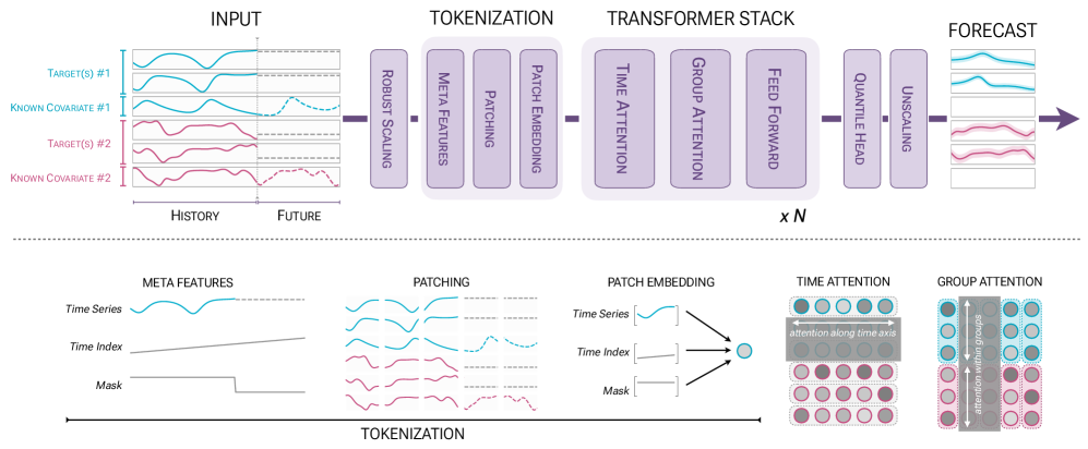
Chronos-2’s core innovation is group attention in the transformer stack. Traditional time series transformers apply self-attention along the temporal dimension. Chronos-2 alternates between two attention mechanisms:

• Time attention: Aggregates information across patches within a single time series (capturing temporal dependencies)
• Group attention: Aggregates information across all series within a group at each patch index (capturing cross-series patterns)

Together with the patching and masking strategy, this mechanism naturally handles diverse scenarios: single time series, multiple series sharing metadata, variates of a multivariate series, or targets with associated covariates. The model infers variable interactions in-context without architectural changes per task.

Critically, compared to concatenating covariates for the multivariate setting (as Moirai-1 does) which leads to quadratic scaling, the group attention mechanism scales linearly with the number of variates $V$.

Since Chronos and GIFT-Eval are primarily univariate corpus datasets, Chronos-2 leverages synthetic data for multivariate capabilities. The training data combines univariate generators (AR models, exponential smoothing, trend-seasonality decompositions) with multivariatizers that impose instantaneous and temporal correlations on sampled univariate series. Combined with curated univariate data, this enables robust cross-task generalization.

Putting Chronos-2 on the test bench: spiking neuron dynamics

Let’s stress-test Chronos-2 on an important problem in neuroscience: neural dynamics. Our goal here is to predict neural firing 🧠🔥.

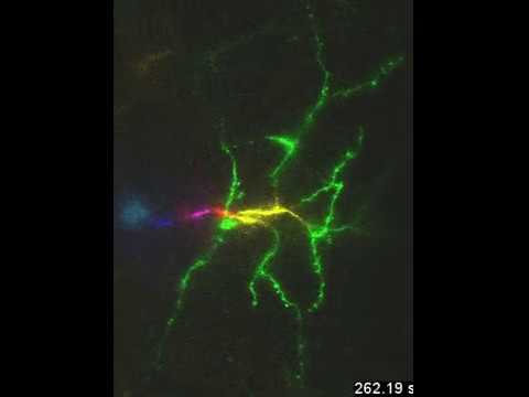
A neuron firing in real-time. Calcium waves sweep along the cell body as the neuron spikes. The complex dynamics we’re trying to predict: can a purely data-driven model forecast when and how these firing patterns emerge? (UC Berkeley images by Na Ji)

We’ll use the FitzHugh-Nagumo model, a simplified neuron model exhibiting complex dynamics from steady states to limit cycles to chaotic attractors. The latter regime echoes the butterfly effect: although the system is fully deterministic, the nonlinearity is such that long-term prediction becomes impossible.

The model describes a neuron’s membrane potential $v$ and recovery variable $w$ driven by external forcing $f(t)$:

$$\frac{dv}{dt} = (1 - v) \cdot v \cdot (v - a) - w + f(t)$$

$$\frac{dw}{dt} = \varepsilon \cdot (v - b \cdot w)$$

We generate diverse time series by varying parameters $a$ (excitability threshold), $b$ (recovery strength), $\varepsilon$ (recovery timescale), and forcing patterns (sinusoidal external stimulus).

This parameter space spans three dynamical regimes: stable fixed points (low excitability), limit cycles (sustained oscillations), and near-chaotic dynamics where long-term prediction becomes infeasible. We test whether Chronos-2 can forecast across these regimes in a zero-shot manner.

Getting Started with Chronos-2

To use Chronos-2, first install the package:

pip install chronos

For basic inference, load the model and call predict_df with your data:

from chronos import BaseChronosPipeline

pipeline = BaseChronosPipeline.from_pretrained(
    "amazon/chronos-2",  # or "autogluon/chronos-2-small" for CPU
    device_map="cuda"     # or "cpu"
)

predictions = pipeline.predict_df(
    context_df,          # Historical data
    prediction_length=H, # Forecast horizon
    id_column='series_id',
    timestamp_column='timestamp',
    target=['y']         # Target variable(s)
)

Check out the quickstart notebook for more comprehensive examples.

Interactive Experiment: Forecasting FitzHugh-Nagumo Dynamics

We created an interactive experiment using Gradio to explore Chronos-2’s capabilities on neural dynamics. The setup simulates multiple FitzHugh-Nagumo time series, which serve as context for cross-learning. One series is held out with specific parameter values to test the model’s zero-shot forecasting ability.

The interface allows adjusting the number of context series for cross-learning, varying FitzHugh-Nagumo parameters ($a$, $b$, $\varepsilon$, forcing amplitude and frequency) to explore different dynamical regimes, and toggling whether the forcing signal is provided as a known covariate. The model forecasts both the membrane potential $v$ and recovery variable $w$ simultaneously (multivariate forecasting) while incorporating the external forcing as a covariate.

Results: Chronos-2 demonstrates impressive forecasting performance across dynamical regimes. When the dynamics exhibit limit cycles, the predictions are nearly indistinguishable from the ground truth. When the system exhibits chaotic behavior (as with the default parameter combination), the model cannot match the ground truth exactly but still captures it accurately over the short to medium term while properly indicating uncertainty in the predictions.

What this means for AI4Science

Chronos-2 enables researchers to establish data-driven performance benchmarks with minimal effort. If Chronos-2 achieves strong predictive performance, your system has learnable structure from data alone. If it fails, you’ve learned something fundamental about intrinsic stochasticity, measurement limitations, or the necessity of domain knowledge. Either way, comparing Chronos-2 against physics-informed models reveals where domain knowledge provides value beyond data. This is scientific insight in itself.

‼️ Important caveat: Ensure your dataset is domain-specific and not represented in pretraining data. While Chronos-2 primarily uses synthetic and public benchmark datasets, verify your application domain wasn’t included in training to avoid inflated performance estimates that would undermine scientific conclusions.

Chronos-2 also supports fine-tuning for developing domain-specific models. Check out the quickstart notebook for examples of covariate-informed forecasting and fine-tuning.

Model weights, code, and documentation available at amazon-science/chronos-forecasting and on the Hugging Face Hub