Changing environments
In this tutorial, we define a birth function that is time dependent. This can be related to changing environment, where the optimal adaptive trait changes because of underlying resource variability, e.g. related to climate.
Defining the variation
  ω = 2* π / 150 # angular frequency
  optimal_trait(t) = sin(ω * t)
  tend = 300
  Plots.plot(1:tend,optimal_trait,label = "Optimal trait",xlabel = "time")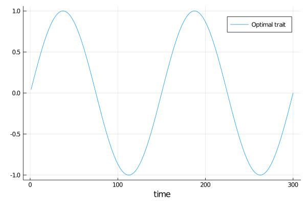
Running
optimal_trait function is fed into the birth function, that we define as gaussian.
myspace = (RealSpace{1,Float64}(),)
K0 = 1000 # We will have in total 1000 individuals
b(X,t) = gaussian(X[1],optimal_trait(t),1)
d(X,Y,t) = 1/K0
D = (5e-2,)
mu = [1.]
NMax = 2000
p = Dict{String,Any}();@pack! p = D,mu,NMax
myagents = [Agent(myspace,(0,),ancestors=true,rates=true) for i in 1:K0]
w0 = World(myagents,myspace,p,0.)
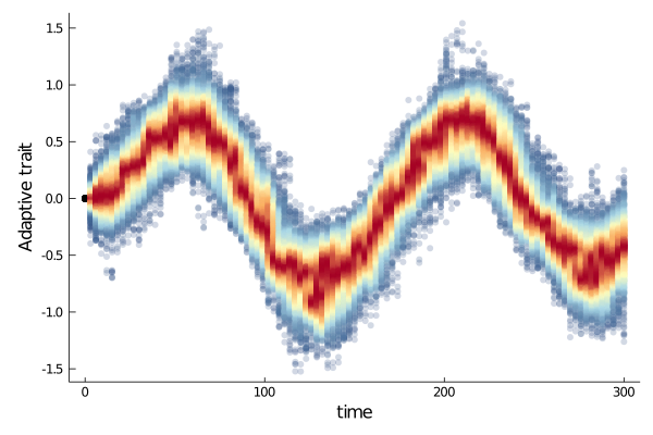
@time sim = run!(w0, Gillepsie(), tend, b, d, dt_saving=3.)Plotting
Plots.plot(sim)