Environmental Gradient

In this tutorial, we model agents evolving on a discrete segment, where each patch favours an optimal adaptive trait, along a gradient. This is typically the case along an altitudinal gradient.

Here is what the geographical space looks like.

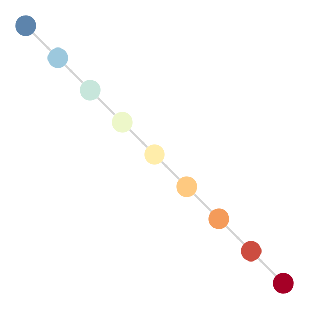
Every colour stands for a different optimal trait.

Run the world

using Revise,ABMEv,Plots,UnPack


nodes = 9
dim_neutr = 30
geospace = DiscreteSegment(Int8(1),Int8(nodes))
adaptivespace = RealSpace{1,Float16}()
myspace = (geospace,adaptivespace)
sigma_K = 1.;
sigma_a = .8;
K0 = 1000;
mu = [1.,1.]
a = 1
b(X,t) = gaussian(X[2],X[1] * a,sigma_K) / nodes
d(X,Y,t) =  (X[1] ≈ Y[1]) * gaussian(X[2],Y[2],sigma_a) / K0
NMax = 2000
D = (5e-1,5e-2)
# tend = 1.5
tend = 1500
p = Dict{String,Any}();@pack! p = NMax,mu,D

myagents = [Agent(myspace,(Int8(5),Float16(5) + Float16(5e-2) * randn(Float16),),ancestors=true,rates=true) for i in 1:round(K0/nodes)]

w0 = World(myagents,myspace,p,0.)

s = run!(w0,Gillepsie(),tend,b,d,dt_saving=5);
Plots.plot(s, ylabel = "Adaptive trait",trait=2)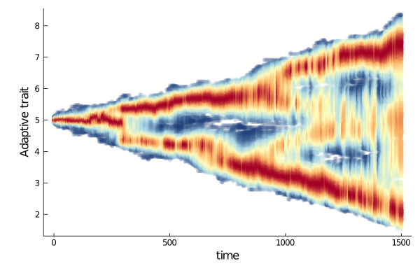

Animated trait space

Here we show how to plot a cool animated scatter plot of the trait space through time.

Plotting lineages

A cool feature of ABMEv.jl is its ability to track agents ancestors traits (cf Agent section)

On can plot it, to get an idea of the coalescence of the population.

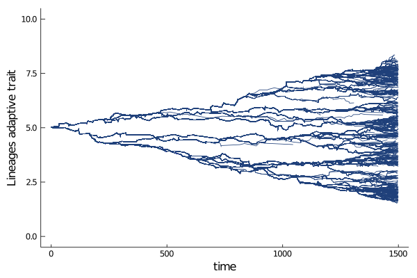
Beautiful, isn't it?